A Hybrid HPC Platform for Dynamic Search in Large Combinatorial Spaces

My BSc thesis in Computer Engineering at Universidad Carlos III de Madrid was carried out at the IQOG-CSIC, with the PNRG group, under David Expósito Singh (UC3M) and Pedro Noheda Marín (IQOG-CSIC). It was graded 9.6/10.

The engineering problem was not the science. It was that the search space the science implies is far too large to enumerate, and the people who needed to explore it needed to do so interactively — steering the search while it ran, rather than submitting a batch job and reading the results the next morning. Those two requirements pull in opposite directions, and the thesis is largely about the architecture that reconciles them.

The result was a hybrid platform: a distributed C++ search engine running on CSIC’s DRAGO supercomputer, coupled to a local interactive tool, with Redis as the coordination boundary between them.

The dataset and the domain-specific scoring functions belong to the PNRG group and are confidential, so this write-up covers the engineering and the measured performance only. The source code was deliberately never published.

1. The problem: why the space explodes

The search runs over subsets of a catalogue of nuclear elements and states. For $n$ items and a set of admissible subset sizes $S$, the space is

\[C_{\text{total}} = \sum_{k \in S} \binom{n}{k}\]

which for the catalogue in question reaches $2^{118} \approx 3.3 \times 10^{35}$ candidates. That is not a number you reduce by being clever about constant factors. Exhaustive enumeration is not a slow strategy, it is a category error.

Each candidate is scored by a set of domain metrics, and the subsets that matter are the ones with extreme or unusual scores. They are rare, unevenly distributed, and — this is the part that drives the whole design — not known in advance. The search cannot be planned at submission time, because where it should go next depends on what it has already found.

A search whose shape is fixed before it starts can be a batch job. A search whose shape depends on intermediate results cannot.

2. Why neither local nor HPC alone was sufficient

Purely local fails on throughput. Scoring candidates is expensive and the work is embarrassingly parallel, so a workstation gives up orders of magnitude the problem could genuinely use.

Purely HPC fails on interaction. A supercomputer is a batch environment: work is queued, scheduled, and run with no human in the loop. Queue latency alone destroys the interaction loop, before considering that compute nodes are not where an exploratory visualisation front-end belongs.

The hybrid design sends the throughput-bound half to DRAGO, keeps the latency-bound, human-facing half local, and pays for a coordination boundary between them.

3. Architecture

The compute side is C++20 with MPI (OpenMPI 4.1.4) across DRAGO’s nodes and OpenMP within each of them, built with GCC 12 at -O3 and scheduled through SLURM. C++20 specifically, because it guarantees atomic fetch_add on floating-point types — which the shared score counters need.

The local side is Python 3.11 for interactive querying and plotting, with the hot paths pushed into C++ extensions through Pybind11 so the same algorithms back both environments.

The platform is three modules, and the split follows the two access patterns rather than any organisational tidiness: one path prepares data once, and two paths consume it very differently.

flowchart LR
    SRC[Source documents] --> M1["<b>Module 1</b><br/>Data extraction"]
    M1 --> PQ[("isotopes.parquet")]
    M1 --> CSV[("isotopes.csv")]
    PQ --> M3["<b>Module 3</b><br/>Dynamic search on HPC<br/><i>C++20 · MPI + OpenMP</i>"]
    CSV --> M2["<b>Module 2</b><br/>Local on-demand tool<br/><i>Python · C++ ext.</i>"]
    M3 --> H5[("HDF5 results<br/>one file per rank")]
    M2 --> VIZ["Plots and views"]

Module 1 runs once and produces a single consolidated file that is the source of truth for both consumers. Module 3 is the throughput path; Module 2 is the latency path. They deliberately share no runtime dependency — the HPC code does not need Python, and the local tool does not need MPI — which is why the same machine never has to satisfy both dependency sets.

Execution lifecycle

flowchart LR
    A["MPI / OpenMP init"] --> B["Read arguments"] --> C["Connect to Redis"]
    C --> D["<b>AdaptiveSearchManager</b><br/><i>what to work on next</i>"]
    D --> E["<b>ScoreEvaluator</b><br/><i>per-candidate scoring</i>"]
    E --> F
    subgraph L["Main search loop &nbsp;·&nbsp; per thread, until regions run out"]
        direction LR
        F["Select<br/>region"] --> G["Process<br/>region"] --> H["Report<br/>score"] --> I["Export<br/>results"]
    end
    F <--> R[("<b>Redis</b><br/>region status · scores")]
    H --> R
    I --> J[("<b>HDF5</b><br/>.rank&lt;N&gt;.h5")]

All ranks load the input, instantiate the two long-lived components, and synchronise on an MPI barrier. The AdaptiveSearchManager owns the decision of what to work on next; the ScoreEvaluator owns the per-candidate computation. Keeping those separate is what makes the scoring swappable without touching the distribution logic.

Each rank then spawns OpenMP threads that loop independently: ask for a region, evaluate every candidate in it, report the score, repeat — until the regions run out. Threads never coordinate with each other directly, and ranks never message each other during the loop; both talk to Redis instead. The loop terminates when the manager reports no regions left or a configured iteration limit is hit, at which point each rank flushes its HDF5 buffers, closes its file, releases Redis and calls MPI_Finalize().

The division of labour is deliberate and worth stating plainly, because each of the three parallelism technologies does exactly one job: MPI for startup, teardown and process topology; OpenMP for saturating the cores inside a node; Redis for every irregular, data-dependent decision in between. Nothing in the hot loop needs a collective, which is why adding nodes costs so little.

Regions and combinatorial indexing

A region is a contiguous block of global lexicographic indices — region $i$ covers indices $[i \cdot R,\ (i+1) \cdot R - 1]$. That definition is what makes the whole thing distributable: a region is fully described by one integer, so handing work to a thread on another node costs nothing.

To make it usable, a thread has to be able to jump straight to an arbitrary index without generating everything before it. That is a combinatorial unranking problem, solved here with binomial counts and a binary mask: locate which subset-size block the global index falls into, subtract the offset, then construct the mask with exactly $K$ bits set corresponding to that rank. The positions of the set bits are the subset.

Unranking is comparatively expensive, so it is used once per region, for the first index; the rest of the block is walked incrementally with a next_comb step. Random access where it is needed, sequential speed everywhere else.

All of this runs on Boost.Multiprecision cpp_int, because 118-bit indices overflow every native integer type available.

Adaptive work distribution

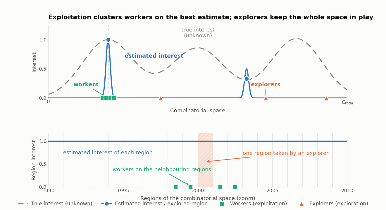
The interesting part is how the next region gets chosen. On each request, the manager assembles a candidate set from two sources: regions neighbouring ones that recently finished (within a window of a few indices, scored by extrapolating from the neighbour and attenuating with distance), and a handful of uniformly random unexplored regions. It then takes the argmax of the estimated score over whatever is still free:

\[r^{*} = \underset{r \in \mathcal{S} \cap \mathcal{A}_t}{\arg\max}\ \hat{s}_r\]

On top of that, a fixed fraction of threads — around 30 % — are designated pure explorers and draw uniformly from the whole space regardless of local scores, so the search cannot collapse into one promising neighbourhood and stay there.

The reason for sampling rather than maintaining global statistics is scale: with $10^{35}$ candidates you cannot keep a visit counter per region. The estimate has to be built from a local sample at the moment of the decision.

4. Storage: Arrow, Parquet and HDF5

Input is Apache Parquet read through Apache Arrow; output is HDF5. Neither is the default choice, and both were argued rather than assumed.

Why not CSV for input. CSV has no schema, no types, no compression, and no structure a reader can exploit — every read is a full parse and every numeric column is a string until proven otherwise. Parquet is columnar and compressed, and Arrow reads it into columnar memory multi-threaded, directly in C++. On DRAGO that matters twice over, because the shared filesystem is Lustre: every rank reads the same consolidated file concurrently, and both layers are built to serve exactly that pattern. CSV was kept only as a secondary export for interoperability.

Why not a relational database. The access pattern is wrong for one. This is bulk append-only analysis: write a great many records, then read whole columns of them. No updates, no transactions worth the name, no joins on the hot path. A DBMS would add an operational dependency and a serialisation bottleneck in exchange for guarantees the workload never uses — and it would have to be reachable from every compute node.

Why HDF5 for output. Results are hierarchical rather than flat: each explored candidate carries scalar scores plus, conditionally, larger derived structures. HDF5 stores that natively — one group per candidate, metrics as attributes, derived structures as datasets, and only the pieces that were actually computed.

The write path is shaped by the parallelism rather than the format. Each rank writes its own file (.rank<N>.h5), which removes inter-process write contention entirely, and within a rank the threads accumulate results in in-memory buffers that are flushed in batches, which keeps I/O off the critical path. Nothing is shared, so nothing needs locking.

5. Coordination through Redis

Redis, via hiredis, is the shared state between processes and nodes. It holds which regions are in progress or finished, per-region scores, and the global counters.

The reservation is the load-bearing part. A thread claims a region with HSETNX — set-if-not-exists, atomic — so two threads on two different nodes cannot take the same region, and no consensus protocol is needed to guarantee it. On finishing, the thread reports the accumulated score, which updates both the region’s status and the sample that feeds later neighbourhood estimates.

The reason this is Redis and not MPI messages is that the assignment pattern is irregular and data-dependent. Expressing “whichever thread finishes first takes the best remaining region” in explicit MPI point-to-point would mean building a distributed work queue by hand. An atomic key-value store already is one.

The same state doubles as a telemetry channel: because progress, scores and per-core position are all already in Redis, a long run can be watched from outside without instrumenting the compute path.

6. Results and performance

Measured on DRAGO — nodes of 2× Intel Xeon (24 cores each, 48 threads per node), 192 GB RAM, Lustre, and a non-blocking Infiniband HDR fat-tree.

Intra-node scaling (OpenMP, fixed problem, one node)

Threads	Time (s)	Speedup	Efficiency
1	657.51	1.00×	100 %
2	158.24	4.16×	208 %
8	37.62	17.48×	218 %
16	17.79	36.97×	231 %
32	10.77	61.06×	191 %
48	9.40	69.93×	146 %

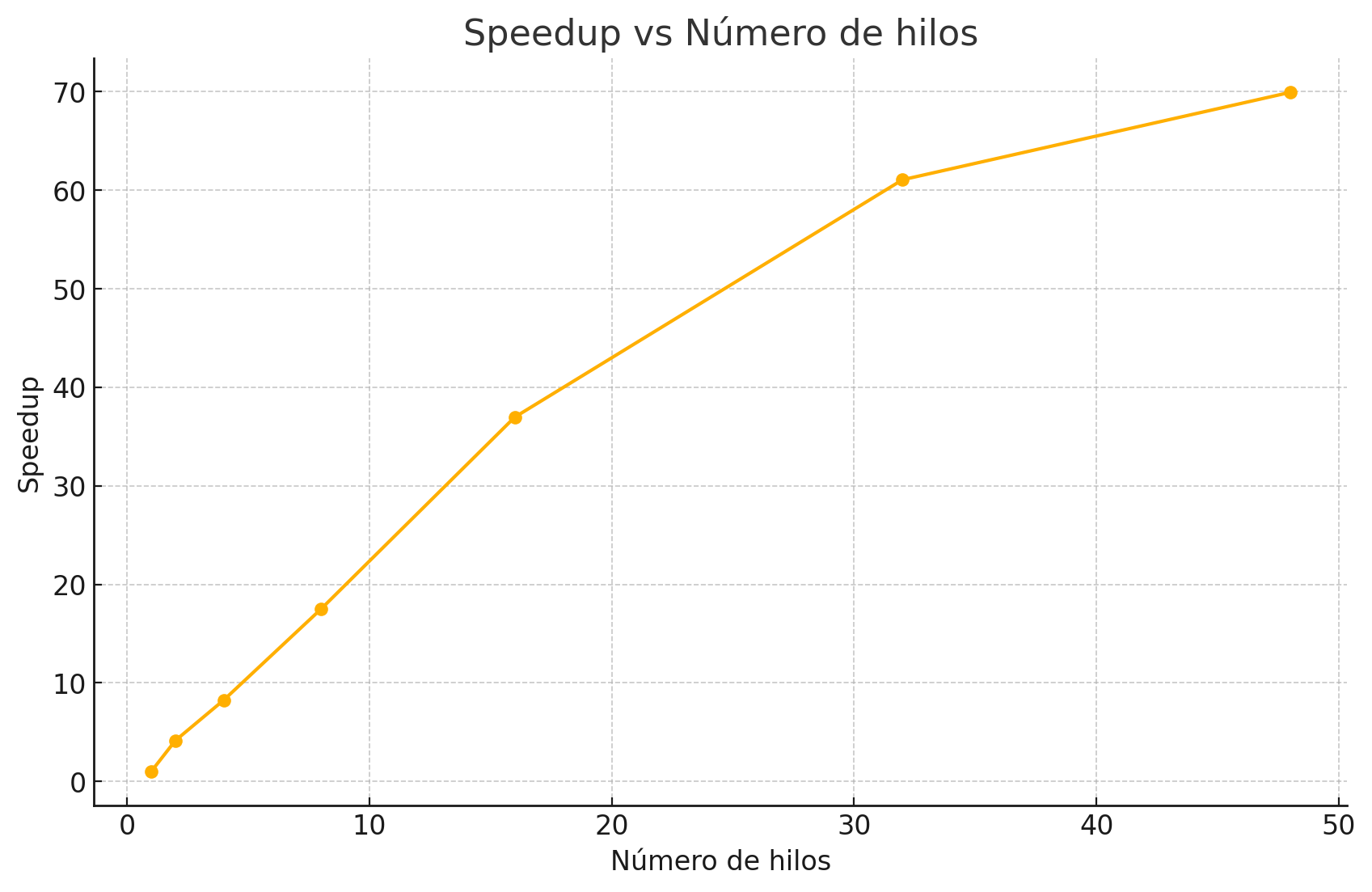Speedup against OpenMP thread count. Axis labels are from the original thesis figures, in Spanish.

The speedup is superlinear up to about 16 threads, peaking at 231 % efficiency. That is not a measurement error: splitting the work shrinks each thread’s working set enough to change its cache behaviour, so the parallel version is doing genuinely cheaper work per candidate, not just more of it at once. Past 32 threads, memory bandwidth and synchronisation overhead take it back — efficiency falls to 146 % at 48 threads, though wall-clock still improves.

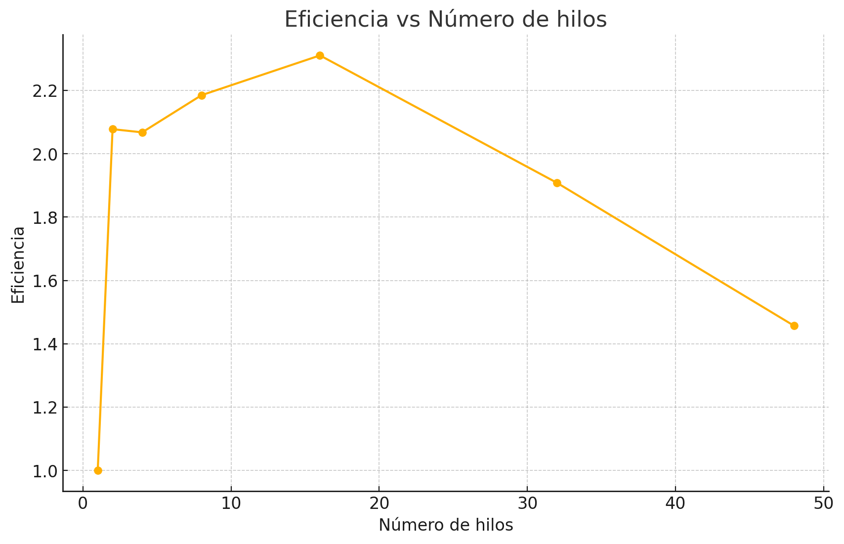Parallel efficiency (speedup ÷ threads) on one node.

The headline: a computation that takes 11 minutes on one thread finishes in 9.4 seconds on a full node.

Multi-node scaling (MPI, 16 threads per node)

Nodes	Total threads	Time (s)	Speedup	Efficiency
1	16	18.22	1.00×	100 %
2	32	9.83	1.85×	92 %
4	64	5.45	3.34×	84 %
8	128	3.01	6.05×	76 %

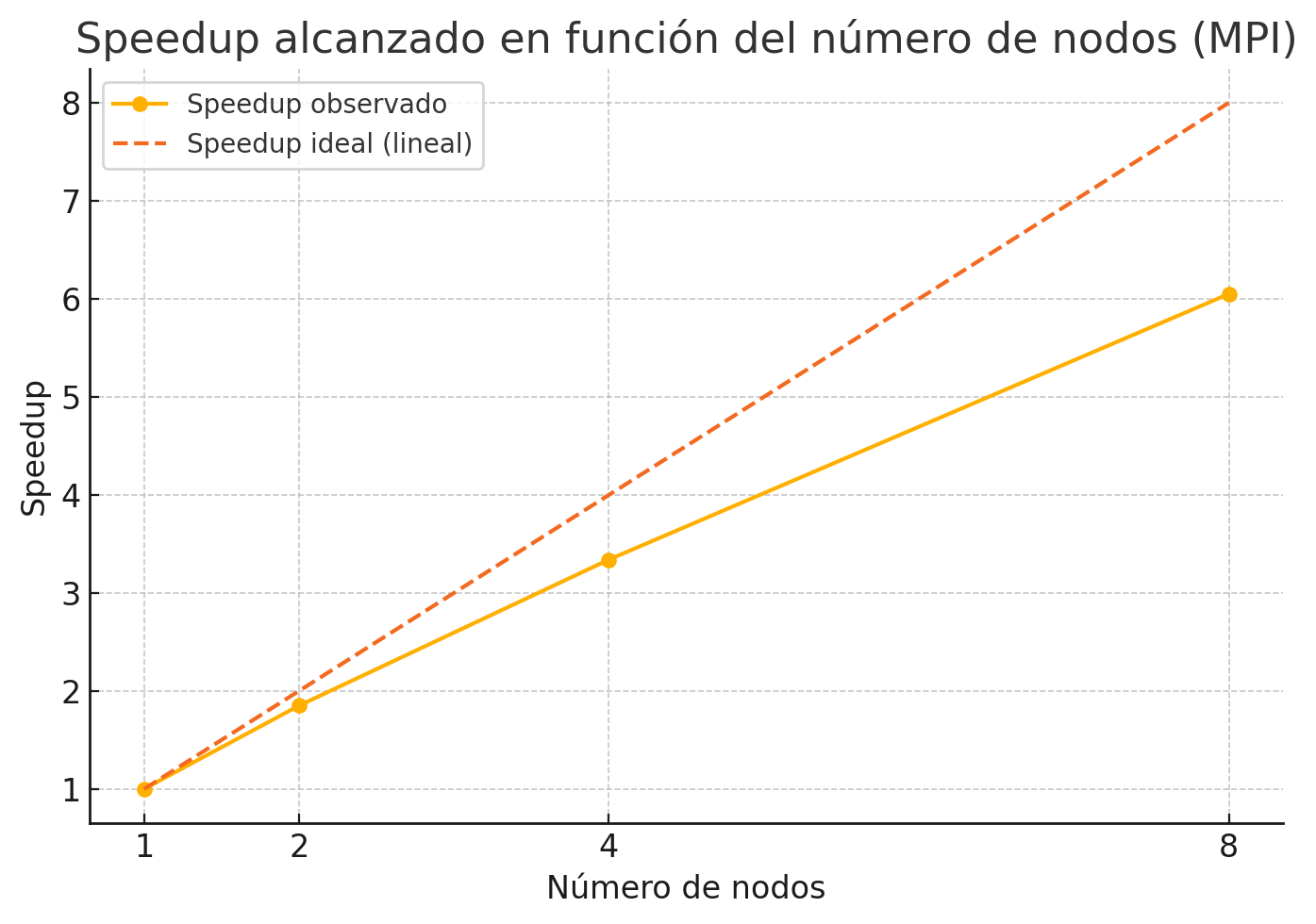Speedup against node count, 16 OpenMP threads per node.

Sublinear, as expected, and the decay is legible: 92 % at two nodes down to 76 % at eight. At eight nodes roughly a quarter of the time is going to coordination rather than computation. Larger node counts were not tested — cluster quota, not a technical limit.

Weak scaling (100k candidates per thread)

Threads	Total candidates	Time (s)	Efficiency
1	100,000	69.6	100 %
2	200,000	33.3	209 %
8	800,000	32.5	214 %
16	1,600,000	33.1	210 %
24	2,400,000	36.5	191 %
32	3,200,000	42.1	165 %
48	4,800,000	54.8	148 %

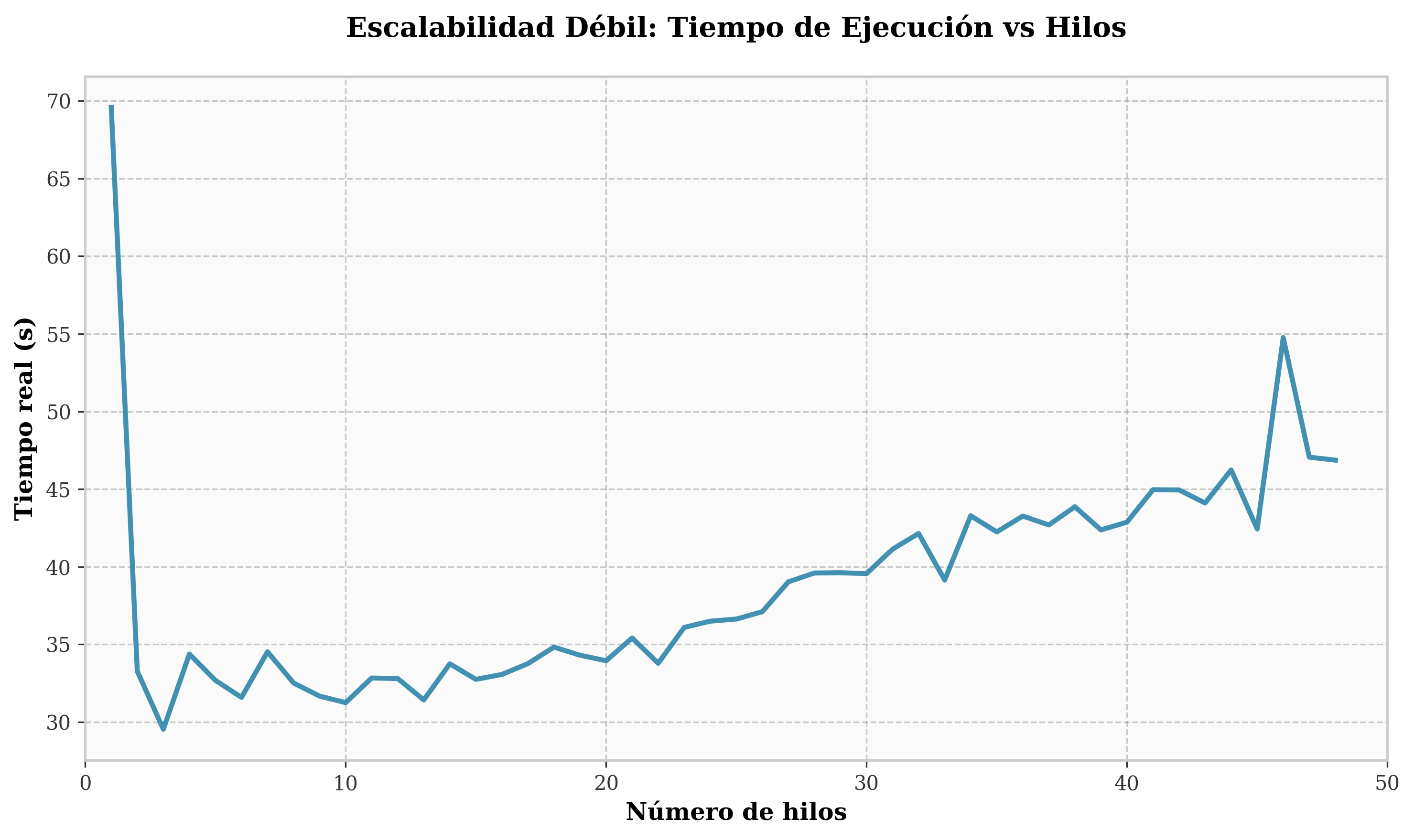Wall-clock time as data and threads grow together.

Wall-clock stays flat around 30–35 seconds from 2 to 16 threads while the workload grows sixteenfold. The extreme point is the one worth quoting: 48 threads processed 48× the data in 54.8 s, against 69.6 s for a single thread on 1/48th of it. More work, less time.

Where the time actually goes

Profiling with gprof produced the most useful result in the whole evaluation, and not a flattering one. With the expensive scoring enabled, 85 % of CPU time was spent in std::vector<>::_M_realloc_insert — reallocating and copying vectors while building intermediate structures. Linear-algebra routines accounted for single-digit percentages; the combinatorial engine barely registered.

With the heavy scoring disabled, the profile flattens into list normalisation (~44 %) and sequence generation (~25 %), which is roughly what you would hope.

So the bottleneck was never the search. It was memory management inside one scoring implementation — a component deliberately designed to be swappable, and one that had been written for correctness with no attention paid to allocation.

7. Observability

Monitoring rode on the coordination layer rather than being built separately. Because region status, scores and progress counters already live in Redis for correctness reasons, an external observer can poll them and watch a long run without touching the compute path or adding instrumentation overhead.

A proper dashboard on top of that — reading Redis and rendering it in Grafana — was designed but not built; it stayed on the future-work list when the project’s hours ran out. Everything it needed was already in the store.

8. What I would do differently today

Some of this I thought at the time. Some only became clear after a year of writing production firmware and then coming back to research.

I would not have hard-coded the tuning parameters. Region size, exploration ratio, neighbourhood window, sample size, buffer sizes — all of them are compile-time constants in the source, and no sensitivity analysis was ever run over them. That is two failures in one: the system cannot be tuned per workload, and I cannot tell you how much of the measured performance is the design versus one lucky guess at a region size. Config file first, then the sweep.

I would take the central coordinator seriously as a scaling limit. Redis was the right call for tens of processes and made the adaptive assignment almost free to implement. But it is a single point every thread contends on, and at hundreds of processes it becomes the bottleneck by construction. A hierarchical scheme — node-local coordinators reconciling against a global one — is the obvious next step, and it is much easier to design in than to retrofit.

I would profile before optimising anything, and I would profile earlier. The 85 % figure is the single most valuable number in the thesis, and I got it near the end. Everything I would have guessed about where the time went was wrong.

I would not store everything. The strategy was to write out every explored candidate for maximum fidelity in later analysis. At this problem’s scale that produces output volumes that become their own engineering problem — a filtering criterion at write time, keeping only candidates that clear a relevance threshold, would have cost almost nothing and saved a great deal.

I would make the extension point actually usable. Adding a new scoring metric requires writing C++ and recompiling the whole thing. For a platform whose users are domain scientists, that is a barrier that decides whether the tool gets adopted at all. A Python or declarative path for metrics, even a slow one, would have been worth more than any of the performance work.

---

Supervised by David Expósito Singh (UC3M) and Pedro Noheda Marín (IQOG-CSIC). Listed on the Publications page.