Forecasting Soil Moisture with LSTMs and Transformers: What the Data Actually Needed
This is the work I did in the GIAA group (Applied Artificial Intelligence) at Universidad Carlos III de Madrid, with the Universidad Politécnica de Madrid, on forecasting soil moisture from a field sensor network. It produced two first-author publications:
- Deep Learning for Robust Soil Moisture Forecasting Using LSTM and Transformer — SOCO 2025, Springer CCIS vol. 2806, pp. 193–202. DOI
- Data-driven forecasting of soil moisture based on enhanced pre-processing of data from on ground sensor networks — Physics and Chemistry of the Earth, Parts A/B/C, vol. 145, art. 104766, 2026. DOI
The obvious post to write about this would be about the models. This is not that post, because the models were not where the difficulty was. The journal title says so out loud — enhanced pre-processing — and that is an honest description of where the contribution sits.
1. Field sensor data is a mess, and that is the actual problem
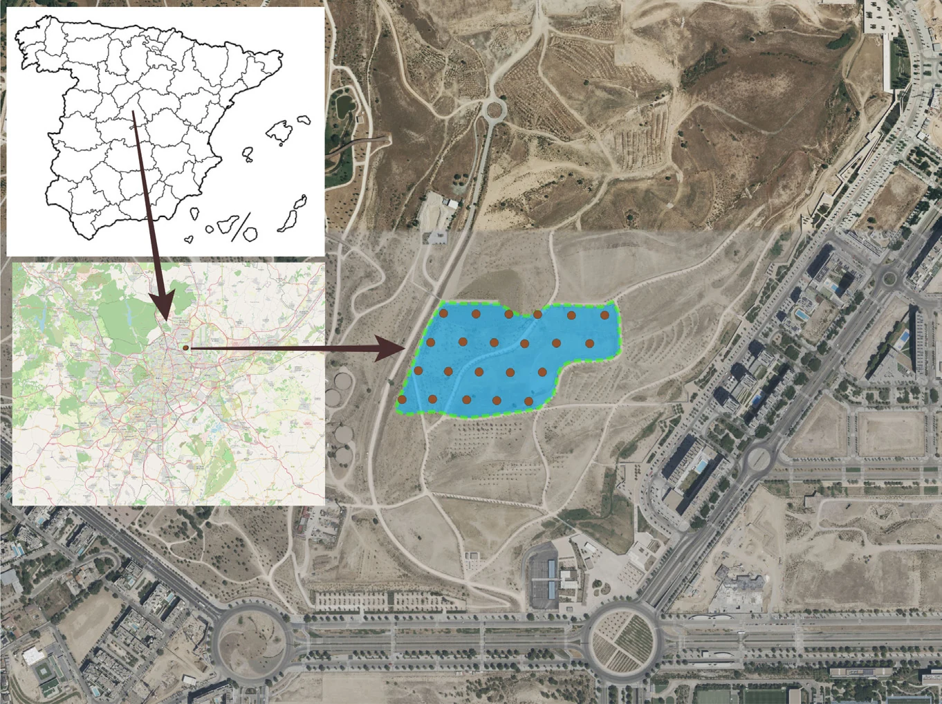
The deployment is a network of 55 soil moisture sensors at the Parque Agrourbano de Valdebebas in Madrid, covering roughly 120,000 m² on a regular 50 × 50 m grid. Each unit is an ESP32-PICO-D4 board with two independent corrosion-resistant resistive probes buried at 10 cm, sampling every 15 minutes, where each recorded value is already the mean of 10 readings.
The header image above is Fig. 1 of the journal paper: the sensor grid sits on the blue polygon, north-east of Madrid. Reproduced from R. Aguilar, M. A. Patricio, A. Berlanga, J. M. Molina and S. Zubelzu, Physics and Chemistry of the Earth, Parts A/B/C 145 (2026) 104766, doi:10.1016/j.pce.2026.104766 — © 2026 Elsevier Ltd, reproduced by the author.
That is a careful design. The data still comes out badly behaved, and the specific ways it fails are worth listing, because they are not the failures a synthetic benchmark prepares you for:
- Batteries fail twice over. Depletion opens gaps while a human goes out to swap cells — but before that, the sensors show a measurable dependence of their output on supply voltage. A draining battery quietly shifts the internal reference, so it produces low-frequency drift and intermittent shutdowns at the same time. The gap is visible; the drift preceding it is not.
- Variance that comes from the electronics, not the soil. The measured value and its variance turn out to be strongly correlated, which is a physical tell: part of the observed variability is amplification behaviour, not soil dynamics. Two probes on the same board can differ in variance by several orders of magnitude.
- The two probes of one device disagree. Within a single physical unit, one channel will show dropouts, offset shifts, isolated peaks or zeros while the other looks fine — transient instability or contact degradation.
- Outliers that are sometimes real. Some spikes are sensor malfunction. Others are heavy rainfall, which is precisely the event the network exists to capture. You cannot filter on shape alone.
None of this is incidental. It is a permanent property of leaving instruments in a field, and any method meant for real data has to survive it.
2. What most papers do about it, and why that is not enough
The standard treatment is brief: drop incomplete records, interpolate small gaps, proceed to the model. Often it goes unmentioned, which amounts to the same thing.
The papers this work builds on generally operate on highly controlled deployments where sensors behave and datasets do not carry corrupted records, so preprocessing is reduced to whatever the chosen algorithm formally requires. That is a reasonable thing to do with good data. It just does not describe the situation of anyone running instruments outdoors.
There are two problems with importing that habit. Dropping incomplete records is not neutral — it removes exactly the periods when the instrumentation was under stress, biasing the training set toward benign conditions and inflating reported performance. And it makes results non-transferable: a model validated on the surviving clean subset has not been shown to work on the data a practitioner actually has.
3. The pipeline selects, it does not repair
Here is the design decision that makes this work different, stated plainly in the paper: the objective was not to correct the raw measurements, but to identify time intervals that were both valid and representative of the underlying soil-moisture dynamics.
That is close to the opposite of the usual instinct. Rather than imputing gaps, smoothing noise and correcting drift — every one of which injects assumptions into the data and then trains a model on them — the pipeline goes looking for stretches of record that were already good, and throws the rest away. What the model sees is original, unmodified measurement.
It runs in three stages.
Stage 1 — Device filtering. Keep only sensors whose records are internally consistent. A device is accepted if it shows no abrupt discontinuity greater than 10 % within any two-hour window (|Δ| > 0.1 normalised, the signature of a sensor or communication failure), has more valid samples than the global mean across all devices (1,391 in this dataset), and shows a Pearson correlation of at least 0.7 between its own two probes. That last one is elegant: the redundant probe is turned into a self-consistency check, so the device certifies itself.
Stage 2 — Interval segmentation and gap detection. Split each surviving series into continuous segments. What counts as a gap was chosen from the physical process that causes gaps: two thresholds were tested, a conservative two days and a permissive five, bracketing how long battery replacement realistically takes across a regular or a long weekend. Segments with fewer than 200 valid measurements are discarded, and only intervals with complete concurrent records of precipitation, temperature, relative humidity, wind velocity and solar radiation survive, since the models are multivariate.
Stage 3 — Interval scoring and selection. Score every remaining segment on duration, sampling density, inter-probe correlation and data quality:
\[\text{Score} = (t_{\text{end}} - t_{\text{start}})^{w_1} \cdot N^{w_2} \cdot |\text{corr}_{12}|^{w_3} \cdot \left(\max\left(0,\ 1 - \frac{f_{o_1} + f_{o_2}}{2}\right)\right)^{w_4} \cdot (\dots)\]where $N$ is the sample count, $\text{corr}{12}$ the correlation between the two probes, and $f{o_j}$ the outlier fraction for probe $j$ by the standard IQR rule. A final term penalises intervals sitting persistently at very low normalised moisture. The score favours long, densely sampled, internally consistent intervals and penalises noisy or flatlined ones.
The five highest-scoring intervals, each from a different device, become the working dataset: 27 to 38 consecutive days, 641 to 908 hourly observations each.
Five intervals out of 55 sensors is a brutal reduction, and the paper is upfront that it costs something — the training set skews toward well-behaved periods and under-represents extreme hydrological events. That is a real limitation, and it is the honest price of not fabricating data.
4. Models, and a baseline that is not a strawman
A broad screen came first, then tuning on whatever looked promising. On the full dataset:
| Model | RMSE | $R^2$ |
|---|---|---|
| Linear regression | 0.0025 | 0.21 |
| Random Forest | 0.0009 | 0.74 |
| SARIMAX | 0.81 | 0.18 |
| LSTM | 0.0010 | 0.72 |
| SARIMAX + RF | 0.002 | 0.27 |
The LSTM and Transformer were then evaluated properly against a simple baseline at 1, 8 and 24 hour horizons, with architectures, hyperparameters and training schedules chosen by Bayesian optimisation (Optuna) with cross-validation. Results averaged over the selected intervals:
| Model | Horizon | RMSE (%) | $R^2$ |
|---|---|---|---|
| LSTM | 1 h | 0.29 ± 0.12 | 0.98 ± 0.02 |
| Transformer | 1 h | 0.37 ± 0.11 | 0.96 ± 0.02 |
| Baseline | 1 h | 0.48 ± 0.09 | 0.93 ± 0.03 |
| LSTM | 8 h | 0.84 ± 0.30 | 0.74 ± 0.14 |
| Transformer | 8 h | 0.69 ± 0.38 | 0.83 ± 0.17 |
| Baseline | 8 h | 1.44 ± 0.42 | 0.25 ± 0.19 |
| LSTM | 24 h | 1.27 ± 0.27 | 0.31 ± 0.20 |
| Transformer | 24 h | 1.10 ± 0.29 | 0.43 ± 0.21 |
| Baseline | 24 h | 1.68 ± 0.20 | −0.46 ± 0.27 |
Two things in that table deserve more attention than they usually get.
At one hour, the baseline gets $R^2 = 0.93$. Soil moisture is heavily autocorrelated, so short-horizon forecasting is close to trivial and a deep model buys you very little. The gap only opens at 8 hours, where the baseline collapses to 0.25 and both deep models hold. Anyone reporting a one-hour result without a persistence baseline is reporting the autocorrelation, not the model.
At 24 hours, everything falls apart — 0.31 and 0.43. The paper draws the correct conclusion rather than the flattering one: making decisions on a 24-hour horizon is not recommended, because soil moisture at that range is not predictable from current observations. The partial autocorrelation function says so directly.
There is one more piece of honesty worth carrying over. A Diebold–Mariano test was run against the baseline, and averaged across lookback windows most of the comparisons do not reach significance — only LSTM-vs-baseline at 24 hours does ($p = 0.005$). The improvements are consistent in direction; the statistical evidence per interval is thinner than the RMSE table alone suggests.
5. What each part contributed
This is the ablation that justifies the framing, and it is why the journal paper is titled the way it is: run only the first two stages of the pipeline instead of all three, and performance degrades.
| Stage run alone | Model | Devices | Max Δ$R^2$ | Max ΔRMSE |
|---|---|---|---|---|
| Device filtering | LSTM | 15 | −0.043 | 0.482 |
| Interval segmentation + gap detection | LSTM | 10 | −0.016 | 1.466 |
| Device filtering | Transformer | 15 | −0.063 | 0.582 |
| Interval segmentation + gap detection | Transformer | 10 | −0.036 | 1.639 |
Meanwhile the scoring weights themselves were varied by up to ±50 % and the selection barely moved — only two intervals changed at the extremes, and downstream performance was essentially unaffected. Only $w_{low}$, the flatline penalty, showed real sensitivity.
That combination is the useful result. The pipeline as a whole matters; the exact weights inside it do not. A practitioner can port the method to their own network without having to replicate a tuning exercise — which is a far more transferable finding than a ranking of architectures.
6. From SOCO 2025 to the journal paper
The conference paper established the approach: the same three-stage philosophy, LSTM and Transformer against a baseline, on the same sensor network. It reported an awkward detail worth preserving — the technical documentation described 55 deployed devices, but the raw data contained 91 unique device identifiers, because device resets change the identifier. Before any modelling, someone had to work out that a third of the “devices” were the same hardware under a new name.
The journal paper extends it in five directions: the scoring function is formalised (Eq. 1) rather than described; the algorithm screen is widened to linear regression, Random Forest and SARIMAX; the Diebold–Mariano significance testing is added; both sensitivity analyses — on the weights and on the pipeline stages — are new, and the second of those is the ablation above; and feature-engineering scenarios are defined and compared explicitly.
In short, SOCO showed the pipeline worked. The journal paper showed which part of it was doing the work, and how much slack there was in the parts that were guessed.
7. Reproducing it
Code is at github.com/Ragarr/soil-moisture-forecasting-lstm-transformer.
The work was funded by the Spanish Ministry of Science and Innovation (PID2023-151605OB-C22) and projects TED2021-131520B-C21 and TED2021-131520B-C22 under the PEICTI 2021–2023 call.
Both papers are listed on the Publications page.